Advanced
The basic interface explained in the Introduction should provide you enough to start detecting communities. However, perhaps you want to improve the partitions further or want to do some more advanced analysis. In this section, we will explain this in more detail.
Optimiser
Although the package provides simple access to the function
find_partition(), there is actually an underlying
Optimiser class that is doing the actual work. We can also
explicitly construct an Optimiser object:
>>> optimiser = louvain.Optimiser()
The function find_partition() then does nothing else then
calling optimise_partition() on the provided
partition.
>>> diff = optimiser.optimise_partition(partition)
But optimise_partition() simply tries to improve any
provided partition. We can thus try to repeatedly call
optimise_partition() to keep on improving the current
partition:
>>> G = ig.Graph.Erdos_Renyi(100, p=5./100)
>>> partition = louvain.ModularityVertexPartition(G)
>>> improv = 1
>>> while improv > 0:
...   improv = optimiser.optimise_partition(partition)
Even if a call to optimise_partition() did not improve
the current partition, it is still possible that a next call will improve the
partition. Of course, if the current partition is already optimal, this will
never happen, but it is not possible to decide whether a partition is optimal.
The optimise_partition() itself is built on a basic
algorithm: move_nodes(). You can also call this
function yourself. For example:
>>> diff = optimiser.move_nodes(partition)
The usual strategy in the Louvain algorithm is then to aggregate the partition
and repeat the move_nodes() on the aggregated
partition. We can easily repeat that:
>>> partition = louvain.ModularityVertexPartition(G)
>>> while optimiser.move_nodes(partition) > 0:
...   partition = partition.aggregate_partition()
This summarises the whole Louvain algorithm in just three lines of code.
Although this finds the final aggregate partition, this leaves it unclear the
actual partition on the level of the individual nodes. In order to do that, we
need to update the membership based on the aggregate partition, for which we
use the function
from_coarse_partition().
>>> partition = louvain.ModularityVertexPartition(G)
>>> partition_agg = partition.aggregate_partition()
>>> while optimiser.move_nodes(partition_agg):
...   partition.from_coarse_partition(partition_agg)
...   partition_agg = partition_agg.aggregate_partition()
Now partition_agg contains the aggregate partition and partition
contains the actual partition of the original graph G. Of course,
partition_agg.quality() == partition.quality() (save some rounding).
The function move_nodes() in turn relies on two key
functions of the partition:
diff_move() and
move_node(). The first
calculates the difference when moving a node, and the latter actually moves the
node, and updates all necessary internal administration. The
move_nodes() then does something as follows
>>> for v in G.vs:
...   best_comm = max(range(len(partition)),
...                   key=lambda c: partition.diff_move(v.index, c))
...   partition.move_node(v.index, best_comm)
The actual implementation is more complicated, but this gives the general idea.
Resolution profile
Some methods accept so-called resolution parameters, such as
CPMVertexPartition or
RBConfigurationVertexPartition. Although some method may seem
to have some ‘natural’ resolution, in reality this is often quite arbitrary.
However, the methods implemented here (which depend in a linear way on
resolution parameters) allow for an effective scanning of a full range for the
resolution parameter. In particular, these methods somehow can be formulated as
\(Q = E - \gamma N\) where \(E\) and \(N\) are some other
quantities. In the case for CPMVertexPartition for example,
\(E = \sum_c m_c\) is the number of internal edges and \(N = \sum_c
\binom{n_c}{2}\) is the sum of the internal possible edges. The essential
insight for these formulations 1 is that if there is an optimal partition
for both \(\gamma_1\) and \(\gamma_2\) then the partition is also
optimal for all \(\gamma_1 \leq \gamma \leq \gamma_2\).
Such a resolution profile can be constructed using the
Optimiser object.
>>> G = ig.Graph.Famous('Zachary')
>>> optimiser = louvain.Optimiser()
>>> profile = optimiser.resolution_profile(G, louvain.CPMVertexPartition,
...                                        resolution_range=(0,1))
Plotting the resolution parameter versus the total number of internal edges we thus obtain something as follows:
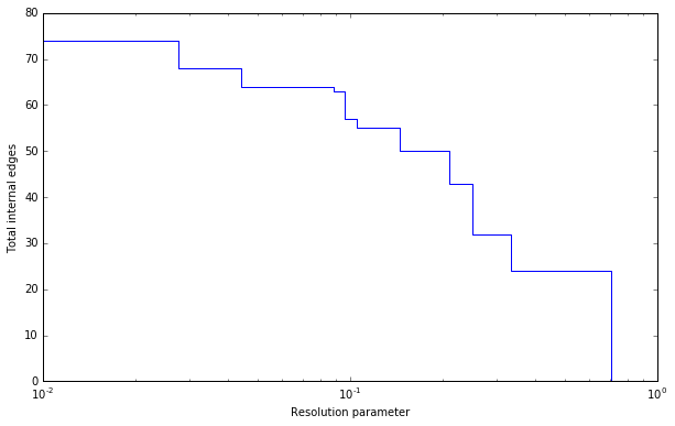
Now profile contains a list of partitions of the specified type
(CPMVertexPartition in this case) for
resolution parameters at which there was a change. In particular,
profile[i] should be better until profile[i+1], or stated otherwise for
any resolution parameter between profile[i].resolution_parameter and
profile[i+1].resolution_parameter the partition at position i should be
better. Of course, there will be some variations because
optimise_partition() will find partitions of varying
quality. The change points can then also vary for different runs.
This function repeatedly calls optimise_partition()
and can therefore require a lot of time. Especially for resolution parameters
right around a change point there may be many possible partitions, thus
requiring a lot of runs.
References
- 1
Traag, V. A., Krings, G., & Van Dooren, P. (2013). Significant scales in community structure. Scientific Reports, 3, 2930. 10.1038/srep02930