Reference¶

Module functions¶

This package implements the louvain algorithm in C++ and exposes it to python. It relies on (python-)igraph for it to function. Besides the relative flexibility of the implementation, it also scales well, and can be run on graphs of millions of nodes (as long as they can fit in memory). Each method is represented by a different class, all of whom derive from MutableVertexPartition. In addition, multiplex graphs are supported as layers, which also supports multislice representations.

Examples

The simplest example just finds a partition using modularity

>>> G = ig.Graph.Tree(100, 3)
>>> partition = louvain.find_partition(G, louvain.ModularityVertexPartition)

Alternatively, one can access the different optimisation routines individually and construct partitions oneself. These partitions can then be optimised by constructing an Optimiser object and running optimise_partition().

>>> G = ig.Graph.Tree(100, 3)
>>> partition = louvain.CPMVertexPartition(G, resolution_parameter = 0.1)
>>> optimiser = louvain.Optimiser()
>>> diff = optimiser.optimise_partition(partition)

The Optimiser class contains also the different subroutines that are used internally by optimise_partition(). In addition, through the Optimiser class there are various options available for changing some of the optimisation procedure which can affect both speed and quality, which are not immediately available in louvain.find_partition().

louvain.find_partition(graph, partition_type, initial_membership=None, weights=None, seed=None, **kwargs)¶

Detect communities using the default settings.

This function detects communities given the specified method in the partition_type. This should be type derived from VertexPartition.MutableVertexPartition, e.g. ModularityVertexPartition or CPMVertexPartition. Optionally an initial membership and edge weights can be provided. Remaining **kwargs are passed on to the constructor of the partition_type, including for example a resolution_parameter.

Parameters

graph (ig.Graph) – The graph for which to detect communities.
partition_type (type of :class:`) – The type of partition to use for optimisation.
initial_membership (list of int) – Initial membership for the partition. If None then defaults to a singleton partition.
weights (list of double, or edge attribute) – Weights of edges. Can be either an iterable or an edge attribute.
seed (int) – Seed for the random number generator. By default uses a random seed if nothing is specified.
**kwargs – Remaining keyword arguments, passed on to constructor of partition_type.

Returns

The optimised partition.

Return type

partition

See also

Optimiser.optimise_partition()

Examples

>>> G = ig.Graph.Famous('Zachary')
>>> partition = louvain.find_partition(G, louvain.ModularityVertexPartition)

louvain.find_partition_multiplex(graphs, partition_type, seed=None, **kwargs)¶

Detect communities for multiplex graphs.

Each graph should be defined on the same set of vertices, only the edges may differ for different graphs. See Optimiser.optimise_partition_multiplex() for a more detailed explanation.

Parameters

graphs (list of ig.Graph) – List of louvain.VertexPartition layers to optimise.
partition_type (type of MutableVertexPartition) – The type of partition to use for optimisation (identical for all graphs).
seed (int) – Seed for the random number generator. By default uses a random seed if nothing is specified.
**kwargs – Remaining keyword arguments, passed on to constructor of partition_type.

Returns

list of int – membership of nodes.
float – Improvement in quality of combined partitions, see Optimiser.optimise_partition_multiplex().

Notes

We don’t return a partition in this case because a partition is always defined on a single graph. We therefore simply return the membership (which is the same for all layers).

Examples

>>> n = 100
>>> G_1 = ig.Graph.Lattice([n], 1)
>>> G_2 = ig.Graph.Lattice([n], 1)
>>> membership, improvement = louvain.find_partition_multiplex([G_1, G_2],
...                                                            louvain.ModularityVertexPartition)

louvain.find_partition_temporal(graphs, partition_type, interslice_weight=1, slice_attr='slice', vertex_id_attr='id', edge_type_attr='type', weight_attr='weight', seed=None, **kwargs)¶

Detect communities for temporal graphs.

Each graph is considered to represent a time slice and does not necessarily need to be defined on the same set of vertices. Nodes in two consecutive slices are identified on the basis of the vertex_id_attr, i.e. if two nodes in two consecutive slices have an identical value of the vertex_id_attr they are coupled. The vertex_id_attr should hence be unique in each slice. The nodes are then coupled with a weight of interslice_weight which is set in the edge attribute weight_attr. No weight is set if the interslice_weight is None (i.e. corresponding in practice with a weight of 1). See time_slices_to_layers() for a more detailed explanation.

Parameters

graphs (list of ig.Graph) – List of louvain.VertexPartition layers to optimise.
partition_type (type of VertexPartition.MutableVertexPartition) – The type of partition to use for optimisation (identical for all graphs).
interslice_weight (float) – The weight of the coupling between two consecutive time slices.
slice_attr (string) – The vertex attribute to use for indicating the slice of a node.
vertex_id_attr (string) – The vertex to use to identify nodes.
edge_type_attr (string) – The edge attribute to use for indicating the type of link (interslice or intraslice).
weight_attr (string) – The edge attribute used to indicate the weight.
seed (int) – Seed for the random number generator. By default uses a random seed if nothing is specified.
**kwargs – Remaining keyword arguments, passed on to constructor of partition_type.

Returns

list of membership – list containing for each slice the membership vector.
float – Improvement in quality of combined partitions, see Optimiser.optimise_partition_multiplex().

Examples

>>> n = 100
>>> G_1 = ig.Graph.Lattice([n], 1)
>>> G_1.vs['id'] = range(n)
>>> G_2 = ig.Graph.Lattice([n], 1)
>>> G_2.vs['id'] = range(n)
>>> membership, improvement = louvain.find_partition_temporal([G_1, G_2],
...                                                           louvain.ModularityVertexPartition,
...                                                           interslice_weight=1)

louvain.slices_to_layers(G_coupling, slice_attr='slice', vertex_id_attr='id', edge_type_attr='type', weight_attr='weight')¶

Convert a coupling graph of slices to layers of graphs.

This function converts a graph of slices to layers so that they can be used with this package. This function assumes that the slices are represented by nodes in G_coupling, and stored in the attribute slice_attr. In other words, G_coupling.vs[slice_attr] should contain ig.Graph s . The slices will be converted to layers, and nodes in different slices will be coupled if the two slices are connected in G_coupling. Nodes in two connected slices are identified on the basis of the vertex_id_attr, i.e. if two nodes in two connected slices have an identical value of the vertex_id_attr they will be coupled. The vertex_id_attr should hence be unique in each slice. The weight of the coupling is determined by the weight of this link in G_coupling, as determined by the weight_attr.

Parameters

G_coupling (ig.Graph) – The graph connecting the different slices.
slice_attr (string) – The vertex attribute which contains the slices.
vertex_id_attr (string) – The vertex attribute which is used to identify whether two nodes in two slices represent the same node, and hence, should be coupled.
edge_type_attr (string) – The edge attribute to use for indicating the type of link (interslice or intraslice).
weight_attr (string) – The edge attribute used to indicate the (coupling) weight.

Returns

G_layers (list of ig.Graph) – A list of slices converted to layers.
G_interslice (ig.Graph) – The interslice coupling layer.
G (ig.Graph) – The complete graph containing all layers and interslice couplings.

Notes

The distinction between slices and layers is not easy to grasp. Slices in this context refer to graphs that somehow represents different aspects of a network. The simplest example is probably slices that represents time: there are different snapshots network across time, and each snapshot is considered a slice. Some nodes may drop out of the network over time, while others enter the network. Edges may change over time, or the weight of the links may change over time. This is just the simplest example of a slice, and there may be different, more complex possibilities. Below an example with three time slices:

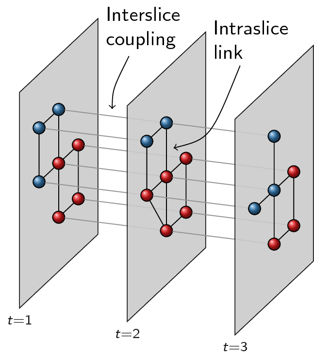
Now in order to optimise partitions across these different slices, we represent them slightly differently, namely as layers. The idea of layers is that all graphs always are defined on the same set of nodes, and that only the links differ for different layers. We thus create new nodes as combinations of original nodes and slices. For example, if node 1 existed in both slice 1 and in slice 2, we will thus create two nodes to build the layers: a node 1-1 and a node 1-2. Additionally, if the slices are connected in the slice graph, the two nodes would also be connected, so there would be a linke between node 1-1 and 1-2. Different slices will then correspond to different layers: each layer only contains the link for that particular slice. In addition, for methods such as CPMVertexPartition, so-called node_sizes are required, and for them to properly function, they should be set to 0 (which is handled appropriately in this function, and stored in the vertex attribute node_size). We thus obtain equally many layers as we have slices, and we need one more layer for representing the interslice couplings. For the example provided above, we thus obtain the following: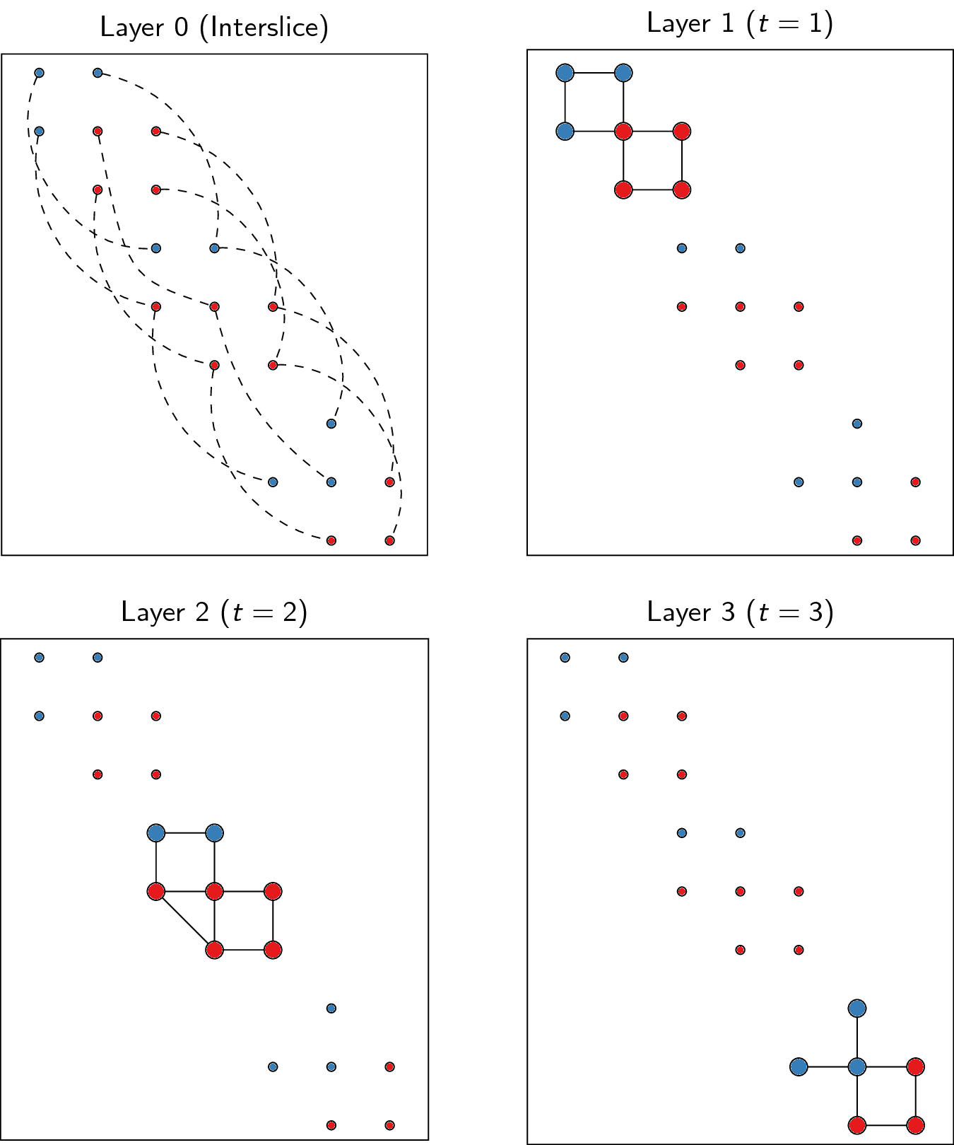

The idea of doing community detection with slices is further detailed in [1].

References

1: Mucha, P. J., Richardson, T., Macon, K., Porter, M. A., & Onnela, J.-P. (2010). Community structure in time-dependent, multiscale, and multiplex networks. Science, 328(5980), 876-8. 10.1126/science.1184819

louvain.time_slices_to_layers(graphs, interslice_weight=1, slice_attr='slice', vertex_id_attr='id', edge_type_attr='type', weight_attr='weight')¶

Convert time slices to layer graphs.

Each graph is considered to represent a time slice. This function simply connects all the consecutive slices (i.e. the slice graph) with an interslice_weight. The further conversion is then delegated to slices_to_layers(), which also provides further details.

Optimiser¶

class louvain.Optimiser¶

Bases: object

Class for doing community detection using the Louvain algorithm.

The optimiser class provides a number of different methods for optimising a given partition. The overall optimise procedure optimise_partition() calls move_nodes() then aggregates the graph and repeats the same procedure. For calculating the actual improvement of moving a node (corresponding a subset of nodes in the aggregate graph), the code relies on diff_move() which provides different values for different methods (e.g. modularity or CPM). Finally, the Optimiser class provides a routine to construct a resolution_profile() on a resolution parameter.

Create a new Optimiser object

property consider_comms¶

Determine how alternative communities are considered for moving a node for optimising a partition.

Nodes will only move to alternative communities that improve the given quality function.

Notes

This attribute should be set to one of the following values

louvain.ALL_NEIGH_COMMS Consider all neighbouring communities for moving.
louvain.ALL_COMMS Consider all communities for moving. This is especially useful in the case of negative links, in which case it may be better to move a node to a non-neighbouring community.
louvain.RAND_NEIGH_COMM Consider a random neighbour community for moving. The probability to choose a community is proportional to the number of neighbours a node has in that community.
louvain.RAND_COMM Consider a random community for moving. The probability to choose a community is proportional to the number of nodes in that community.

property consider_empty_community¶

if True consider also moving nodes to an empty community (default).

Type: boolean

move_nodes(partition, consider_comms=None)¶

Move nodes to alternative communities for optimising the partition.

Parameters

partition – The partition for which to move nodes.
consider_comms – If None uses consider_comms, but can be set to something else.

Returns

Improvement in quality function.

Return type

float

Notes

When moving nodes, the function loops over nodes and considers moving the node to an alternative community. Which community depends on consider_comms. The function terminates when no more nodes can be moved to an alternative community.

Examples

>>> G = ig.Graph.Famous('Zachary')
>>> optimiser = louvain.Optimiser()
>>> partition = louvain.ModularityVertexPartition(G)
>>> diff = optimiser.move_nodes(partition)

optimise_partition(partition)¶

Optimise the given partition.

Parameters: partition – The MutableVertexPartition to optimise.
Returns: Improvement in quality function.
Return type: float

Examples

>>> G = ig.Graph.Famous('Zachary')
>>> optimiser = louvain.Optimiser()
>>> partition = louvain.ModularityVertexPartition(G)
>>> diff = optimiser.optimise_partition(partition)

optimise_partition_multiplex(partitions, layer_weights=None)¶

Optimise the given partitions simultaneously.

Parameters

partitions – List of MutableVertexPartition layers to optimise.
layer_weights – List of weights of layers.

Returns

Improvement in quality of combined partitions, see Notes.

Return type

float

Notes

This method assumes that the partitions are defined for graphs with the same vertices. The connections between the vertices may be different, but the vertices themselves should be identical. In other words, all vertices should have identical indices in all graphs (i.e. node i is assumed to be the same node in all graphs). The quality of the overall partition is simply the sum of the individual qualities for the various partitions, weighted by the layer_weight. If we denote by \(Q_k\) the quality of layer \(k\) and the weight by \(\lambda_k\), the overall quality is then

\[Q = \sum_k \lambda_k Q_k.\]

This is particularly useful for graphs containing negative links. When separating the graph in two graphs, the one containing only the positive links, and the other only the negative link, by supplying a negative weight to the latter layer, we try to find relatively many positive links within a community and relatively many negative links between communities. Note that in this case it may be better to assign a node to a community to which it is not connected so that consider_comms may be better set to louvain.ALL_COMMS.

Besides multiplex graphs where each node is assumed to have a single community, it is also useful in the case of for example multiple time slices, or in situations where nodes can have different communities in different slices. The package includes some special helper functions for using optimise_partition_multiplex() in such cases, where there is a conversion required from (time) slices to layers suitable for use in this function.

Examples

>>> G_pos = ig.Graph.SBM(100, pref_matrix=[[0.5, 0.1], [0.1, 0.5]], block_sizes=[50, 50])
>>> G_neg = ig.Graph.SBM(100, pref_matrix=[[0.1, 0.5], [0.5, 0.1]], block_sizes=[50, 50])
>>> optimiser = louvain.Optimiser()
>>> partition_pos = louvain.ModularityVertexPartition(G_pos)
>>> partition_neg = louvain.ModularityVertexPartition(G_neg)
>>> diff = optimiser.optimise_partition_multiplex(
...                     partitions=[partition_pos, partition_neg],
...                     layer_weights=[1,-1])

resolution_profile(graph, partition_type, resolution_range, weights=None, bisect_func=<function Optimiser.<lambda>>, min_diff_bisect_value=1, min_diff_resolution=0.001, linear_bisection=False, number_iterations=1, **kwargs)¶

Use bisectioning on the resolution parameter in order to construct a resolution profile.

Parameters

graph – The graph for which to construct a resolution profile.
partition_type – The type of MutableVertexPartition used to find a partition (must support resolution parameters obviously).
resolution_range – The range of resolution values that we would like to scan.
weights – If provided, indicates the edge attribute to use as a weight.
bisect_func – The function used for bisectioning. For the methods currently implemented, this should usually not be altered.
min_diff_bisect_value – The difference in the value returned by the bisect_func below which the bisectioning stops (i.e. by default, a difference of a single edge does not trigger further bisectioning).
min_diff_resolution – The difference in resolution below which the bisectioning stops. For positive differences, the logarithmic difference is used by default, i.e. diff = log(res_1) - log(res_2) = log(res_1/res_2), for which diff > min_diff_resolution to continue bisectioning. Set the linear_bisection to true in order to use only linear bisectioning (in the case of negative resolution parameters for example, which can happen with negative weights).
linear_bisection – Whether the bisectioning will be done on a linear or on a logarithmic basis (if possible).
number_iterations – Indicates the number of iterations of the algorithm to run. If negative (or zero) the algorithm is run until a stable iteration.

Returns

A list of partitions for different resolutions.

Return type

list of MutableVertexPartition

Examples

>>> G = ig.Graph.Famous('Zachary')
>>> optimiser = louvain.Optimiser()
>>> profile = optimiser.resolution_profile(G, louvain.CPMVertexPartition,
...                                        resolution_range=(0,1))

set_rng_seed(value)¶

Set the random seed for the random number generator.

Parameters: value – The integer seed used in the random number generator

MutableVertexPartition¶

class louvain.VertexPartition.MutableVertexPartition(graph, initial_membership=None)¶

Bases: VertexClustering

Contains a partition of graph, derives from ig.VertexClustering.

This class contains the basic implementation for optimising a partition. Specifically, it implements all the administration necessary to keep track of the partition from various points of view. Internally, it keeps track of the number of internal edges (or total weight), the size of the communities, the total incoming degree (or weight) for a community, et cetera.

In order to keep the administration up-to-date, all changes in a partition should be done through move_node() or set_membership(). The first moves a node from one community to another, and updates the administration. The latter simply updates the membership vector and updates the administration.

The basic idea is that diff_move() computes the difference in the quality function if we would call move_node() for the same move. These functions are overridden in any derived classes to provide an actual implementation. These functions are used by Optimiser to optimise the partition.

Warning

This base class should never be used in practice, since only derived classes provide an actual implementation.

Parameters

graph – The ig.Graph on which this partition is defined.
membership – The membership vector of this partition. Membership[i] = c implies that node i is in community c. If None, it is initialised with a singleton partition community, i.e. membership[i] = i.

classmethod FromPartition(partition, **kwargs)¶

Create a new partition from an existing partition.

Parameters

partition – The MutableVertexPartition to replicate.
**kwargs – Any remaining keyword arguments will be passed on to the constructor of the new partition.

Notes

This may for example come in handy when determining the quality of a partition using a different method. Suppose that we already have a partition p and that we want to determine the Significance of that partition. We can then simply use

>>> p = louvain.find_partition(ig.Graph.Famous('Zachary'),
...                            louvain.ModularityVertexPartition)
>>> sig = louvain.SignificanceVertexPartition.FromPartition(p).quality()

aggregate_partition(membership_partition=None)¶

Aggregate the graph according to the current partition and provide a default partition for it.

The aggregated graph can then be found as a parameter of the partition partition.graph.

Notes

This function contrasts to the function cluster_graph in igraph itself, which also provides the aggregate graph, but we may require setting the appropriate resolution_parameter, weights and node_sizes. In particular, this function also ensures that the quality defined on the aggregate partition is identical to the quality defined on the original partition.

Examples

>>> G = ig.Graph.Famous('Zachary')
>>> partition = louvain.find_partition(G, louvain.ModularityVertexPartition)
>>> aggregate_partition = partition.aggregate_partition(partition)
>>> aggregate_graph = aggregate_partition.graph
>>> aggregate_partition.quality() == partition.quality()
True

diff_move(v, new_comm)¶

Calculate the difference in the quality function if node v is moved to community new_comm.

Parameters

v – The node to move.
new_comm – The community to move to.

Returns

Difference in quality function.

Return type

float

Notes

The difference returned by diff_move should be equivalent to first determining the quality of the partition, then calling move_node, and then determining again the quality of the partition and looking at the difference. In other words

>>> partition = louvain.find_partition(ig.Graph.Famous('Zachary'),
...                            louvain.ModularityVertexPartition)
>>> diff = partition.diff_move(v=0, new_comm=0)
>>> q1 = partition.quality()
>>> partition.move_node(v=0, new_comm=0)
>>> q2 = partition.quality()
>>> round(diff, 10) == round(q2 - q1, 10)
True

Warning

Only derived classes provide actual implementations, the base class provides no implementation for this function.

from_coarse_partition(partition, coarse_node=None)¶

Update current partition according to coarser partition.

Parameters

partition (MutableVertexPartition) – The coarser partition used to update the current partition.
coarse_node (list of int) – The coarser node which represent the current node in the partition.

Notes

This function is to be used to determine the correct partition for an aggregated graph. In particular, suppose we move nodes and then get an aggregate graph.

>>> diff = optimiser.move_nodes(partition)
>>> aggregate_partition = partition.aggregate_partition()

Now we also move nodes in the aggregate partition

>>> diff = optimiser.move_nodes(aggregate_partition)

Now we improved the quality function of aggregate_partition, but this is not yet reflected in the original partition. We can thus call

>>> partition.from_coarse_partition(aggregate_partition)

so that partition now reflects the changes made to aggregate_partition.

The coarse_node can be used it the aggregate_partition is not defined based on the membership of this partition. In particular the membership of this partition is defined as follows:

>>> for v in G.vs:
...   partition.membership[v] = aggregate_partition.membership[coarse_node[v]] 

If coarse_node is None it is assumed the coarse node was defined based on the membership of the current partition, so that

>>> for v in G.vs:
...   partition.membership[v] = aggregate_partition.membership[partition.membership[v]] 

This can be useful when the aggregate partition is defined on a more refined partition.

move_node(v, new_comm)¶

Move node v to community new_comm.

Parameters

v – Node to move.
new_comm – Community to move to.

Examples

>>> G = ig.Graph.Famous('Zachary')
>>> partition = louvain.ModularityVertexPartition(G)
>>> partition.move_node(0, 1)

quality()¶: The current quality of the partition.

renumber_communities()¶

Renumber the communities so that they are numbered in decreasing size.

Notes

The sort is not necessarily stable.

set_membership(membership)¶: Set membership.

total_possible_edges_in_all_comms()¶

The total possible number of edges in all communities.

Notes

If we denote by \(n_c\) the number of nodes in community \(c\), this is simply

\[\sum_c \binom{n_c}{2}\]

total_weight_from_comm(comm)¶

The total weight (i.e. number of edges) from a community.

Parameters: comm – Community

Notes

This includes all edges, also the ones that are internal to a community. Sometimes this is also referred to as the community (out)degree.

See also

total_weight_to_comm(), total_weight_in_comm(), total_weight_in_all_comms()

total_weight_in_all_comms()¶

The total weight (i.e. number of edges) within all communities.

Notes

This should be equal to simply the sum of total_weight_in_comm for all communities.

See also

total_weight_to_comm(), total_weight_from_comm(), total_weight_in_comm()

total_weight_in_comm(comm)¶

The total weight (i.e. number of edges) within a community.

Parameters: comm – Community

See also

total_weight_to_comm(), total_weight_from_comm(), total_weight_in_all_comms()

total_weight_to_comm(comm)¶

The total weight (i.e. number of edges) to a community.

Parameters: comm – Community

Notes

This includes all edges, also the ones that are internal to a community. Sometimes this is also referred to as the community (in)degree.

See also

total_weight_from_comm(), total_weight_in_comm(), total_weight_in_all_comms()

weight_from_comm(v, comm)¶: The total number of edges (or sum of weights) to node v from community comm.

See also

weight_to_comm()

weight_to_comm(v, comm)¶: The total number of edges (or sum of weights) from node v to community comm.

See also

weight_from_comm()

ModularityVertexPartition¶

class louvain.ModularityVertexPartition(graph, initial_membership=None, weights=None)¶

Bases: MutableVertexPartition

Implements modularity.

Notes

The quality function is

\[Q = \frac{1}{2m} \sum_{ij} \left(A_{ij} - \frac{k_i k_j}{2m} \right)\delta(\sigma_i, \sigma_j)\]

where \(A\) is the adjacency matrix, \(k_i\) is the degree of node \(i\), \(m\) is the total number of edges, \(\sigma_i\) denotes the community of node \(i\) and \(\delta(\sigma_i, \sigma_j) = 1\) if \(\sigma_i = \sigma_j\) and 0 otherwise.

This can alternatively be formulated as a sum over communities:

\[Q = \frac{1}{2m} \sum_{c} \left(m_c - \frac{K_c^2}{4m} \right)\]

where \(m_c\) is the number of internal edges of community \(c\) and \(K_c = \sum_{i \mid \sigma_i = c} k_i\) is the total degree of nodes in community \(c\).

References

1: Newman, M. E. J., & Girvan, M. (2004). Finding and evaluating community structure in networks. Physical Review E, 69(2), 026113. 10.1103/PhysRevE.69.026113

Parameters

graph (ig.Graph) – Graph to define the partition on.
initial_membership (list of int) – Initial membership for the partition. If None then defaults to a singleton partition.
weights (list of double, or edge attribute) – Weights of edges. Can be either an iterable or an edge attribute.

RBConfigurationVertexPartition¶

class louvain.RBConfigurationVertexPartition(graph, initial_membership=None, weights=None, resolution_parameter=1.0)¶

Bases: LinearResolutionParameterVertexPartition

Implements Reichardt and Bornholdt’s Potts model with a configuration null model.

This quality function uses a linear resolution parameter.

Notes

The quality function is

\[Q = \sum_{ij} \left(A_{ij} - \gamma \frac{k_i k_j}{2m} \right)\delta(\sigma_i, \sigma_j)\]

where \(A\) is the adjacency matrix, \(k_i\) is the degree of node \(i\), \(m\) is the total number of edges, \(\sigma_i\) denotes the community of node \(i\), \(\delta(\sigma_i, \sigma_j) = 1\) if \(\sigma_i = \sigma_j\) and 0 otherwise, and, finally \(\gamma\) is a resolution parameter.

This can alternatively be formulated as a sum over communities:

\[Q = \sum_{c} \left(m_c - \gamma\frac{K_c^2}{4m} \right)\]

where \(m_c\) is the number of internal edges of community \(c\) and \(K_c = \sum_{i \mid \sigma_i = c} k_i\) is the total degree of nodes in community \(c\).

Note that this is the same as ModularityVertexPartition for \(\gamma=1\) and using the normalisation by \(2m\).

References

1: Reichardt, J., & Bornholdt, S. (2006). Statistical mechanics of community detection. Physical Review E, 74(1), 016110. 10.1103/PhysRevE.74.016110

Parameters

graph (ig.Graph) – Graph to define the partition on.
initial_membership (list of int) – Initial membership for the partition. If None then defaults to a singleton partition.
weights (list of double, or edge attribute) – Weights of edges. Can be either an iterable or an edge attribute.
resolution_parameter (double) – Resolution parameter.

property resolution_parameter¶: Resolution parameter.

RBERVertexPartition¶

class louvain.RBERVertexPartition(graph, initial_membership=None, weights=None, node_sizes=None, resolution_parameter=1.0)¶

Bases: LinearResolutionParameterVertexPartition

Implements Reichardt and Bornholdt’s Potts model with a configuration null model.

This quality function uses a linear resolution parameter.

Notes

The quality function is

\[Q = \sum_{ij} \left(A_{ij} - \gamma p \right)\delta(\sigma_i, \sigma_j)\]

where \(A\) is the adjacency matrix,

\[p = \frac{m}{\binom{n}{2}}\]

is the overall density of the graph, \(\sigma_i\) denotes the community of node \(i\), \(\delta(\sigma_i, \sigma_j) = 1\) if \(\sigma_i = \sigma_j\) and 0 otherwise, and, finally \(\gamma\) is a resolution parameter.

This can alternatively be formulated as a sum over communities:

\[Q = \sum_{c} \left[m_c - \gamma p \binom{n_c}{2} \right]\]

where \(m_c\) is the number of internal edges of community \(c\) and \(n_c\) the number of nodes in community \(c\).

References

1: Reichardt, J., & Bornholdt, S. (2006). Statistical mechanics of community detection. Physical Review E, 74(1), 016110. 10.1103/PhysRevE.74.016110

Parameters

graph (ig.Graph) – Graph to define the partition on.
initial_membership (list of int) – Initial membership for the partition. If None then defaults to a singleton partition.
weights (list of double, or edge attribute) – Weights of edges. Can be either an iterable or an edge attribute.
node_sizes (list of int, or vertex attribute) – Sizes of nodes are necessary to know the size of communities in aggregate graphs. Usually this is set to 1 for all nodes, but in specific cases this could be changed.
resolution_parameter (double) – Resolution parameter.

CPMVertexPartition¶

class louvain.CPMVertexPartition(graph, initial_membership=None, weights=None, node_sizes=None, resolution_parameter=1.0)¶

Bases: LinearResolutionParameterVertexPartition

Implements CPM. This quality function uses a linear resolution parameter.

Notes

The quality function is

\[Q = \sum_{ij} \left(A_{ij} - \gamma \right)\delta(\sigma_i, \sigma_j)\]

where \(A\) is the adjacency matrix, \(\sigma_i\) denotes the community of node \(i\), \(\delta(\sigma_i, \sigma_j) = 1\) if \(\sigma_i = \sigma_j\) and 0 otherwise, and, finally \(\gamma\) is a resolution parameter.

This can alternatively be formulated as a sum over communities:

\[Q = \sum_{c} \left[m_c - \gamma \binom{n_c}{2} \right]\]

where \(m_c\) is the number of internal edges of community \(c\) and \(n_c\) the number of nodes in community \(c\).

The resolution parameter \(\gamma\) for this functions has a particularly simple interpretation. The internal density of communities

\[p_c = \frac{m_c}{\binom{n_c}{2}} \geq \gamma\]

is higher than \(\gamma\), while the external density

\[p_{cd} = \frac{m_{cd}}{n_c n_d} \leq \gamma\]

is lower than \(\gamma\). In other words, choosing a particular \(\gamma\) corresponds to choosing to find communities of a particular density, and as such defines communities. Finally, the definition of a community is in a sense independent of the actual graph, which is not the case for any of the other methods (see the reference for more detail).

References

1: Traag, V. A., Van Dooren, P., & Nesterov, Y. (2011). Narrow scope for resolution-limit-free community detection. Physical Review E, 84(1), 016114. 10.1103/PhysRevE.84.016114

Parameters

graph (ig.Graph) – Graph to define the partition on.
initial_membership (list of int) – Initial membership for the partition. If None then defaults to a singleton partition.
weights (list of double, or edge attribute) – Weights of edges. Can be either an iterable or an edge attribute.
node_sizes (list of int, or vertex attribute) – Sizes of nodes are necessary to know the size of communities in aggregate graphs. Usually this is set to 1 for all nodes, but in specific cases this could be changed.
resolution_parameter (double) – Resolution parameter.

Bipartite(resolution_parameter_01, resolution_parameter_0=0, resolution_parameter_1=0, degree_as_node_size=False, types='type', **kwargs)¶

Create three layers for bipartite partitions.

This creates three layers for bipartite partition necessary for detecting communities in bipartite networks. These three layers should be passed to Optimiser.optimise_partition_multiplex() with layer_weights=[1,-1,-1].

Parameters

graph (ig.Graph) – Graph to define the bipartite partitions on.
resolution_parameter_01 (double) – Resolution parameter for in between two classes.
resolution_parameter_0 (double) – Resolution parameter for class 0.
resolution_parameter_1 (double) – Resolution parameter for class 1.
degree_as_node_size (boolean) –
If True use degree as node size instead of 1, to mimic modularity, see Notes.
types (vertex attribute or list) – Indicator of the class for each vertex. If not 0, 1, it is automatically converted.
**kwargs – Additional arguments passed on to default constructor of CPMVertexPartition.
_notes-bipartite (..) –

Notes

For bipartite networks, we would like to be able to set three different resolution parameters: one for within each class \(\gamma_0, \gamma_1\), and one for the links between classes, \(\gamma_{01}\). Then the formulation would be

\[Q = \sum_{ij} [A_{ij} - (\gamma_0\delta(s_i,0) + \gamma_1\delta(s_i,1)) \delta(s_i,s_j) - \gamma_{01}(1 - \delta(s_i, s_j)) ]\delta(\sigma_i, \sigma_j)\]

In terms of communities this is

\[Q = \sum_c (e_c - \gamma_{01} 2 n_c(0) n_c(1) - \gamma_0 n^2_c(0) - \gamma_1 n^2_c(1))\]

where \(n_c(0)\) is the number of nodes in community \(c\) of class 0 (and similarly for 1) and \(e_c\) is the number of edges within community \(c\). We denote by \(n_c = n_c(0) + n_c(1)\) the total number of nodes in community \(c\).

We achieve this by creating three layers : (1) all nodes have node_size = 1 and all relevant links; (2) only nodes of class 0 have node_size = 1 and no links; (3) only nodes of class 1 have node_size = 1 and no links. If we add the first with resolution parameter \(\gamma_{01}\), and the others with resolution parameters \(\gamma_{01} - \gamma_0\) and \(\gamma_{01} - \gamma_1\), but the latter two with a layer weight of -1 while the first layer has layer weight 1, we obtain the following:

\[\begin{split}Q &= \sum_c (e_c - \gamma_{01} n_c^2) -\sum_c (- (\gamma_{01} - \gamma_0) n_c(0)^2) -\sum_c (- (\gamma_{01} - \gamma_1) n_c(1)^2) \\ &= \sum_c [e_c - \gamma_{01} 2 n_c(0) n_c(1) - \gamma_{01} n_c(0)^2 - \gamma_{01} n_c(1)^2) + ( \gamma_{01} - \gamma_0) n_c(0)^2 + ( \gamma_{01} - \gamma_1) n_c(1)^2 ] \\ &= \sum_c [e_c - \gamma_{01} 2 n_c(0) n_c(1) - \gamma_{0} n_c(0)^2 - \gamma_{1} n_c(1)^2]\end{split}\]

Although the derivation above is using \(n_c^2\), implicitly assuming a direct graph with self-loops, similar derivations can be made for undirected graphs using \(\binom{n_c}{2}\), but the notation is then somewhat more convoluted.

If we set node sizes equal to the degree, we get something similar to modularity, except that the resolution parameter should still be divided by \(2m\). In particular, in general (i.e. not specifically for bipartite graph) if node_sizes=G.degree() we then obtain

\[Q = \sum_{ij} A_{ij} - \gamma k_i k_j\]

In the case of bipartite graphs something similar is obtained, but then correctly adapted (as long as the resolution parameter is also appropriately rescaled).

Note

This function is not suited for directed graphs in the case of using the degree as node sizes.

SignificanceVertexPartition¶

class louvain.SignificanceVertexPartition(graph, initial_membership=None, node_sizes=None)¶

Bases: MutableVertexPartition

Implements Significance.

Notes

The quality function is

\[Q = \sum_c \binom{n_c}{2} D(p_c \parallel p)\]

where \(n_c\) is the number of nodes in community \(c\),

\[p_c = \frac{m_c}{\binom{n_c}{2}},\]

is the density of community \(c\),

\[p = \frac{m}{\binom{n}{2}}\]

is the overall density of the graph, and finally

\[D(x \parallel y) = x \ln \frac{x}{y} + (1 - x) \ln \frac{1 - x}{1 - y}\]

is the binary Kullback-Leibler divergence.

For directed graphs simply multiply the binomials by 2. The expected Significance in Erdos-Renyi graphs behaves roughly as \(\frac{1}{2} n \ln n\) for both directed and undirected graphs in this formulation.

Warning

This method is not suitable for weighted graphs.

References

1: Traag, V. A., Krings, G., & Van Dooren, P. (2013). Significant scales in community structure. Scientific Reports, 3, 2930. 10.1038/srep02930

Parameters

graph (ig.Graph) – Graph to define the partition on.
initial_membership (list of int) – Initial membership for the partition. If None then defaults to a singleton partition.
node_sizes (list of int, or vertex attribute) – Sizes of nodes are necessary to know the size of communities in aggregate graphs. Usually this is set to 1 for all nodes, but in specific cases this could be changed.

SurpriseVertexPartition¶

class louvain.SurpriseVertexPartition(graph, initial_membership=None, weights=None, node_sizes=None)¶

Bases: MutableVertexPartition

Implements (asymptotic) Surprise.

Notes

The quality function is

\[Q = m D(q \parallel \langle q \rangle)\]

where \(m\) is the number of edges,

\[q = \frac{\sum_c m_c}{m},\]

is the fraction of internal edges,

\[\langle q \rangle = \frac{\sum_c \binom{n_c}{2}}{\binom{n}{2}}\]

is the expected fraction of internal edges, and finally

\[D(x \parallel y) = x \ln \frac{x}{y} + (1 - x) \ln \frac{1 - x}{1 - y}\]

is the binary Kullback-Leibler divergence.

For directed graphs we can multiplying the binomials by 2, and this leaves \(\langle q \rangle\) unchanged, so that we can simply use the same formulation. For weighted graphs we can simply count the total internal weight instead of the total number of edges for \(q\), while \(\langle q \rangle\) remains unchanged.

References

1: Traag, V. A., Aldecoa, R., & Delvenne, J.-C. (2015). Detecting communities using asymptotical surprise. Physical Review E, 92(2), 022816. 10.1103/PhysRevE.92.022816

Parameters

graph (ig.Graph) – Graph to define the partition on.
initial_membership (list of int) – Initial membership for the partition. If None then defaults to a singleton partition.
weights (list of double, or edge attribute) – Weights of edges. Can be either an iterable or an edge attribute.
node_sizes (list of int, or vertex attribute) – Sizes of nodes are necessary to know the size of communities in aggregate graphs. Usually this is set to 1 for all nodes, but in specific cases this could be changed.